I was was a little confused on when to expect a “lateral” velocity in the vehicle body frame after analyzing some GPS speed data one day. I thought that the center of the vehicle shouldn’t have any lateral velocity unless the vehicle is slipping, which for a small and slow golfcart is reasonable to assume. But that’s not the case, and I’ll show a gif to prove it.

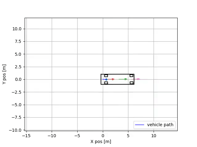
I wanted to come up with a graphic that shows you the different velocity vectors at different points along the vehicles longitudinal axis. You can read my motivation for creating this graphic below, or you could just look at the gif. I’ll leave it up to you.

Background

The gold standard for consulting vehicle dynamics has generally been Rajesh Rajamni’s Vehicle Dynamics and Control. In Chapter Two, he defines the 3DOF kinematic equations of motions as:

Note I made some simplifications that the vehicle is front steered only, and has wheelbase L

\[\dot{X} = V\cos(\theta + \beta)\] \[\dot{Y} = V\sin(\theta + \beta)\] \[\dot{\theta} = V\frac{\cos(\beta)}{L} \tan{\delta}\] \[\beta = \arctan{\dfrac{\tan{\delta}}{2}}\]

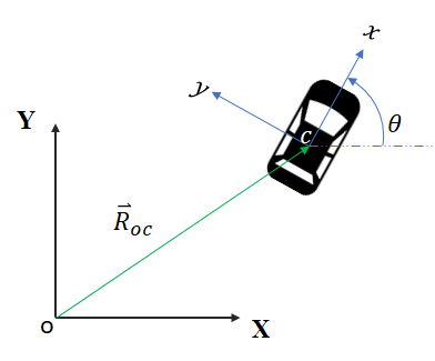
with \(\beta\) as defined as the “vehicle side slip”. \(X , Y\) are the inertial/global co-ordinates at the vehicle center, \(\theta\) the vehicle yaw, and \(\delta\) the steering input angle.

Making a mistake

I also looked at another few literature sources for the kinematic car model, and saw that they had some simplified equations, shown below. I really wasn’t paying attention to their derivation, and thought that they must have set \(\beta = 0\) from Rajamani’s equations due to a assumption of little vehicle side slip.

\[\dot{X} = V\cos(\theta)\] \[\dot{Y} = V\sin(\theta)\] \[\dot{\theta} = V\frac{\tan{\delta}}{L}\]

I thought “okay, I don’t have to really worry about side slip since I have a small and slow moving vehicle, so I’ll too just set \(\beta = 0\)“.

So one day, when trying to find the components of the velocity in the body frame, I used a transformation matrix and came up with:

\[\begin{bmatrix} v_{x} \\ v_{y} \end{bmatrix} = \begin{bmatrix} \cos(\theta) & \sin(\theta) \\ -\sin(\theta) & \cos(\theta) \end{bmatrix} \begin{bmatrix} \dot{X} \\ \dot{Y} \end{bmatrix}\]

Solving this out, I discovered \(v_y\) was zero at the center of the vehicle! I didn’t really think about it until one day I was trying to figure out why some IMU/GPS data was giving me such a large component in the body \(y\) direction after transforming it.

Why \(v_y\) is not zero at the center

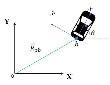
So remember how I set \(\beta = 0\)? Yeah, you can’t do that. That’s not what those other papers did. Although you actually end up with some valid equations of motion, they are only valid at the rear center-point on the axle, like shown below. I figured this out by looking at the side-slip equation one more time, and realized it was actually just a kinematic constraint. I was conflating the vehicle side slip with “tire side slip”.

Retrospectively, this is a silly mistake and am kinda embarrassed to post this; but hopefully this post may guide another confused person (or me again) in the future.

So what does this mean physically?

So \(V_y\) is actually zero still, just at the rear midpoint of the vehicles axle. Of course, if you have a larger/faster vehicle, then this probably won’t be true anymore.